Batch vs Mini-batch vs Stochastic Gradient Descent with Code Examples

What is the difference between these three Gradient Descent variants?

One of the main questions that arises when studying Machine Learning and Deep Learning is the several types of Grandient Descent. Should I use Batch Gradient Descent? Mini-batch Gradient Descent or Stochastic Gradient Descent? In this post we are going to understand the difference between those concepts and take a look in code implementations from Gradient Descent, for the purpose of clarifying these methods.

At this point, we know that our matrix of weights W and our vector of bias b are the core values of our Neural Networks (NN) (Check the Deep Learning Basics post). We can make an analogy with these concepts with the memory in which a NN stores patterns, and it is through tuning these parameters that we teach a NN. The acting of tuning this is done through the optimization algorithms, the amazing feature that allows NN to learn. After some time training the network, these patterns are learned and we have a set of weights and biases that hopefully correct classifies the inputs.

Gradient Descent

One of the most common algorithms that help the NN to reach the correct values of weights and bias. The Gradient Descent (GD) is a method/algorithm to minimize the cost function J(W,b) in each step. It iteratively updates the weights and bias trying to reach the global minimum in a cost function.

Minimizing the Cost Function, a Gradient Descent Illustration. Source: Stanford’s Andrew Ng’s MOOC Machine Learning Course

Review this quickly, before we can compute the GD, first the inputs are taken and passed through all the nodes of a neural network, calculating the weighted sum of inputs, weights, and bias. This first pass is one of the main steps when calculating Gradient Descent and it is called Forward Propagation. Once we have an output, we compare this output with the expected output and calculate how far it is from each other, the error. With this error, we can now propagate it backward, updating each and every weight and bias and trying to minimize this error. And this part is called, as you may anticipate, Backward Propagation. The Backward Propagation step is calculated using derivatives and return the “gradients”, values that tell us in which direction we should follow to minimize the cost function.

We are now ready to update the weight matrix W and the bias vector b. The gradient descent rule is as follows:

In other words, the new weight/bias value will be the last one minus the gradient, moving it close to the global minimum value of the cost function. We also multiply this gradient to a learning rate alpha, which controls how big the step would be. For a more deep approach to Forward and Backward Propagation, Compute Losses, Gradient Descent, check this post.

This classic Gradient Descent is also called Batch Gradient Descent. In this method, every epoch runs through all the training dataset, to only then calculate the loss and update the W and b values. Although it provides stable convergence and a stable error, this method uses the entire training set; hence it is very slow for big datasets.

Mini-batch Gradient Descent

Imagine taking your dataset and dividing it into several chunks, or batches. So instead of waiting until the algorithm runs through the entire dataset to only after update the weights and bias, it updates at the end of each, so-called, mini-batch. This allows us to move quickly to the global minimum in the cost function and update the weights and biases multiple times per epoch now. The most common mini-batch sizes are 16, 32, 64, 128, 256, and 512. Most of the projects use Mini-batch GD because it is faster in larger datasets.

X = data_input
Y = labels
parameters = initialize_parameters(layers_dims)

for i in range(0, num_iterations):
	
	minibatches = random_mini_batches(X, Y, mini_batch_size)

	for minibatch in minibatches:

	    # Select a minibatch
	    (minibatch_X, minibatch_Y) = minibatch
	    # Forward propagation
	    a, caches = forward_propagation(X, parameters)
	    # Compute cost.
	    cost += compute_cost(a, Y)
	    # Backward propagation.
	    grads = backward_propagation(a, caches, parameters)
	    # Update parameters.
	    parameters = update_parameters(parameters, grads)

To prepare the mini-batches, one most apply some preprocessing steps: randomizing the dataset in order to random split the dataset and then partitioning it in the right number of chunks. But what happens if we chose to set the number of batches to 1 or equal to the number of training examples?

Batch Gradient Descent

As stated before, in this gradient descent, each batch is equal to the entire dataset. That is:

Where {1} denotes the first batch from the mini-batch. The downside is that it takes too long per iteration. This method can be used to training datasets with less than 2000 training examples.

X = data_input
Y = labels
parameters = initialize_parameters(layers_dims)
for i in range(0, num_iterations):
    # Forward propagation
    a, caches = forward_propagation(X, parameters)
    # Compute cost
    cost += compute_cost(a, Y)
    # Backward propagation.
    grads = backward_propagation(a, caches, parameters)
    # Update parameters.
    parameters = update_parameters(parameters, grads)

Stochastic Gradient Descent

On other hand, in this method, each batch is equal to one example from the training set. In this example, the first mini-batch is equal to the first training example:

Where (1) denotes the first training example. Here the downside is that it loses the advantage gained from vectorization, has more oscilation but converges faster.

X = data_input
Y = labels
parameters = initialize_parameters(layers_dims)
for i in range(0, num_iterations):
    for j in range(0, m):
        # Forward propagation
        a, caches = forward_propagation(X[:,j], parameters)
        # Compute cost
        cost += compute_cost(a, Y[:,j])
        # Backward propagation
        grads = backward_propagation(a, caches, parameters)
        # Update parameters.
        parameters = update_parameters(parameters, grads)

Summary

It is essential to understand the difference between these optimization algorithms, as they compose a key function for Neural Networks. In summary, although Batch GD has higher accuracy than Stochastic GD, the latter is faster. The middle ground of the two and the most adopted, Mini-batch GD, combine both to deliver good accuracy and good performance.

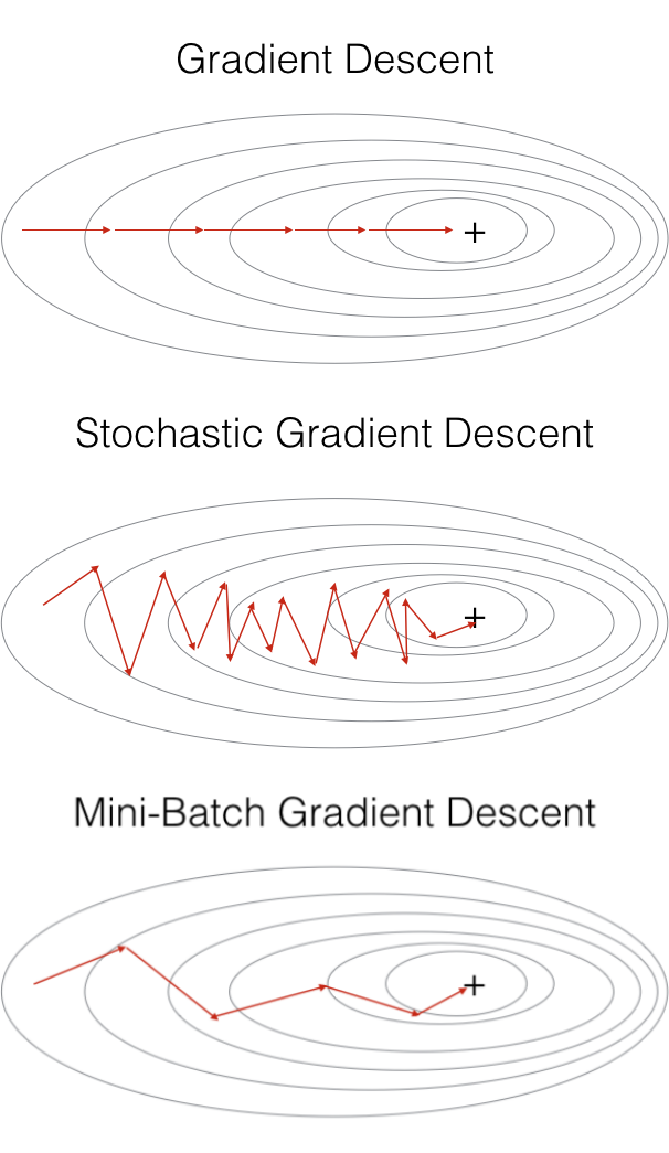
Batch vs Stochastic vs Mini-batch Gradient Descent. Source: Stanford’s Andrew Ng’s MOOC Deep Learning Course

It is possible to use only the Mini-batch Gradient Descent code to implement all versions of Gradient Descent, you just need to set the mini_batch_size equals one to Stochastic GD or to the number of training examples to Batch GD. Thus, the main difference between Batch, Mini-batch and Stochastic Gradient Descent is the number of examples used for each epoch and the time and effort necessary to reach the global minimum value of the Cost Function.